Stabilize the variance
The loss is computed after a Generalized Anscombe Transform, so faint veils and bright cores weigh the same in the fit.
Denoising with no training data. A randomly-initialized neural network is fitted to your single linear image and stopped at the exact moment it has learned the structure but not yet the noise. Nothing can be hallucinated from a training set that does not exist.
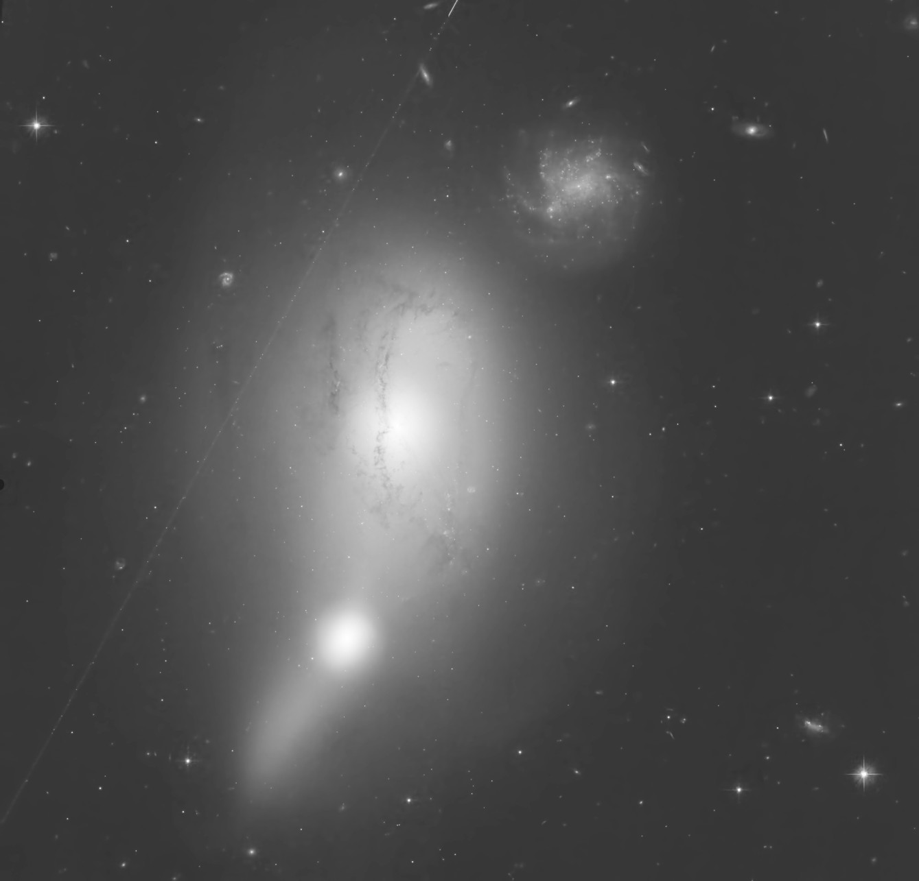
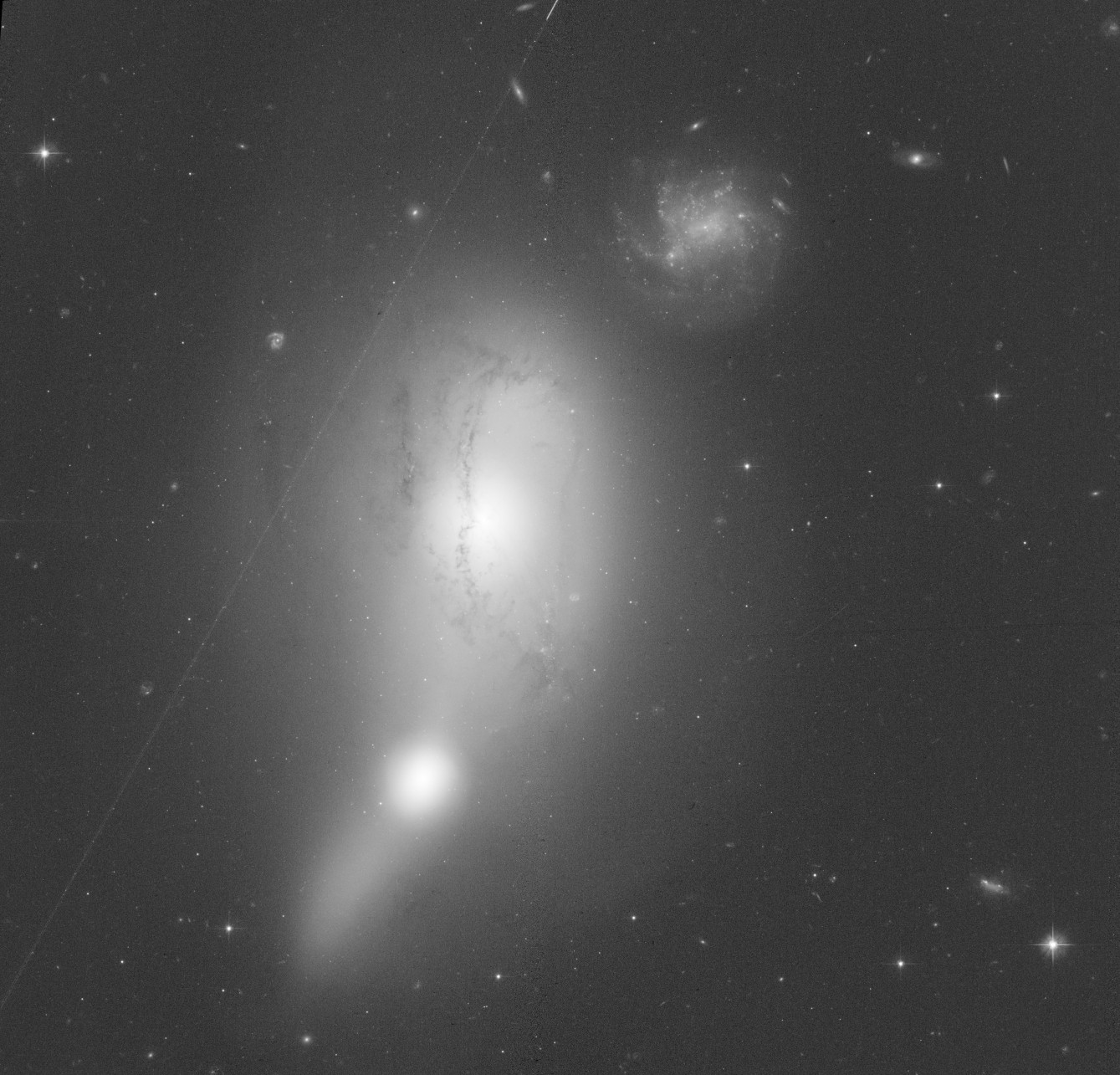
Drag across the image to compare. Two 390 s F606W exposures, 15.5 megapixels, denoised in one full-frame fit. Both sides share the same display stretch, computed on the input. The background galaxies come out of the grain, and the satellite trail crossing the field survives untouched: real structure stays, only the noise goes.
 Input
DIPL
Input
DIPL
Every AI denoiser you know is a network trained on thousands of images: it denoises your picture with priors learned from other people's pictures. Deep Image Prior (Ulyanov et al. 2018) has no training set at all. The network starts from random weights and is fitted, from scratch, to your single image. Real structure gets learned fast, noise gets learned slow. Stop at the right moment and the noise never makes it in.
On linear astronomical data the textbook method breaks three ways. The loss only sees the bright pixels. The noise is Poisson-Gaussian, not white. And there is no ground truth to tell you when to stop, which with this method is everything. For seven years it only ever worked on stretched images and small crops.
The loss is computed after a Generalized Anscombe Transform, so faint veils and bright cores weigh the same in the fit.
No tiles, no seams: the whole image gets one coherent optimization. A 16 Mpx frame needs a datacenter GPU; smaller images run on consumer hardware.
ES-WMV (Wang et al. 2023) watches the moving variance of the output itself and detects the structure-to-noise transition, plus a warm-up guard against false early minima.
Pure DIP output looks synthetic. The final image is
0.55*denoised + 0.45*original in linear space: natural grain, photometry safe.
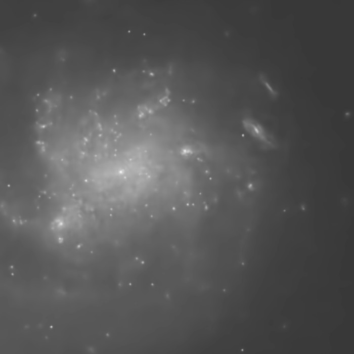
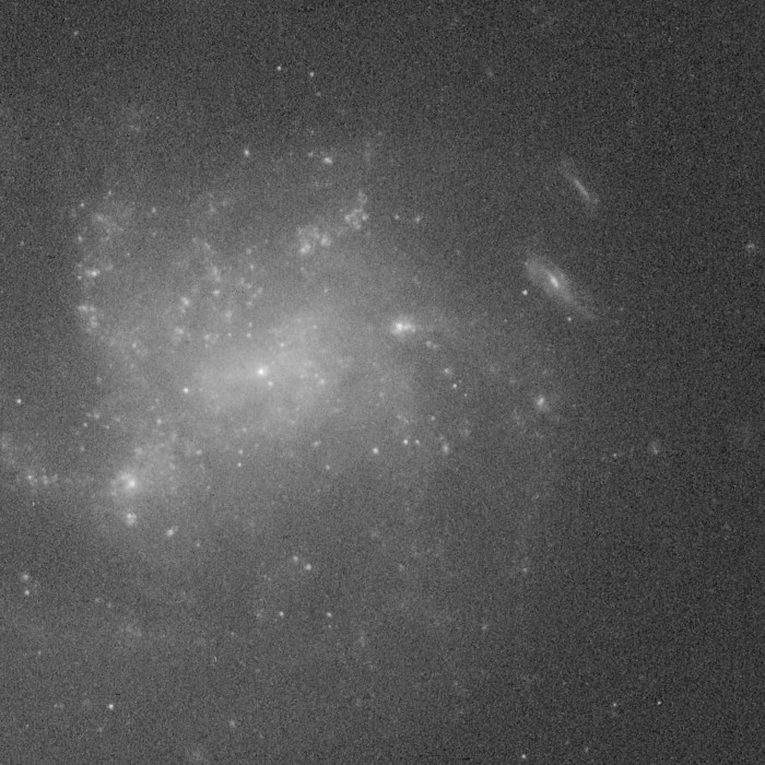
A 700 px crop at native HST resolution on the clumpy satellite of NGC 4933. The star-forming knots come out of the grain one by one, and the two edge-on background galaxies sharpen up. This field is the hardest of the series: it used the full 25 000-iteration budget.
One honest detail: at 1:1 scale the very faintest stars can fade in the pure DIPL output, because point sources at the noise level are the last thing the network learns. More iterations bring them back, and the final blend re-injects part of them anyway.
 Input
DIPL
Input
DIPL
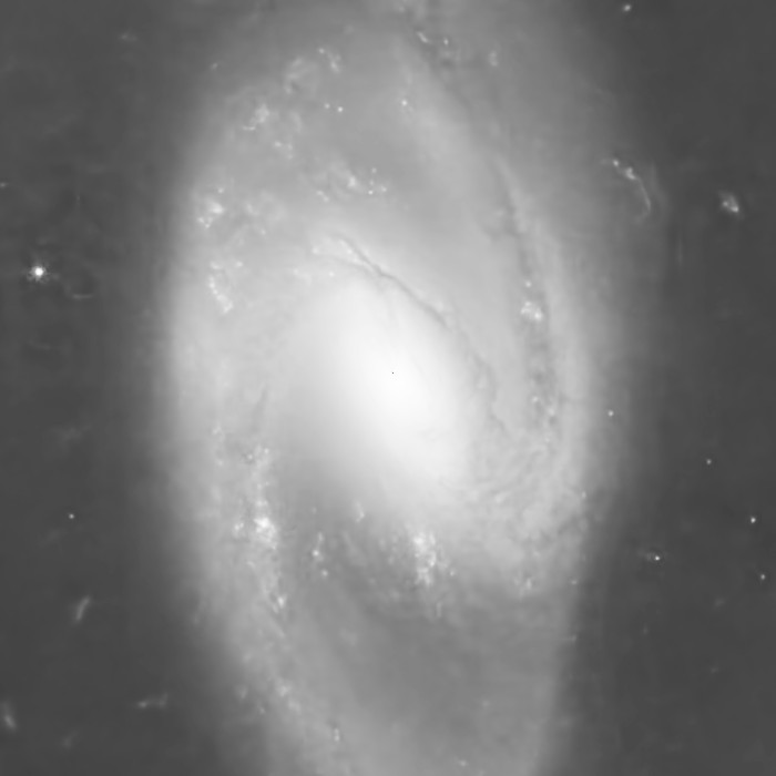
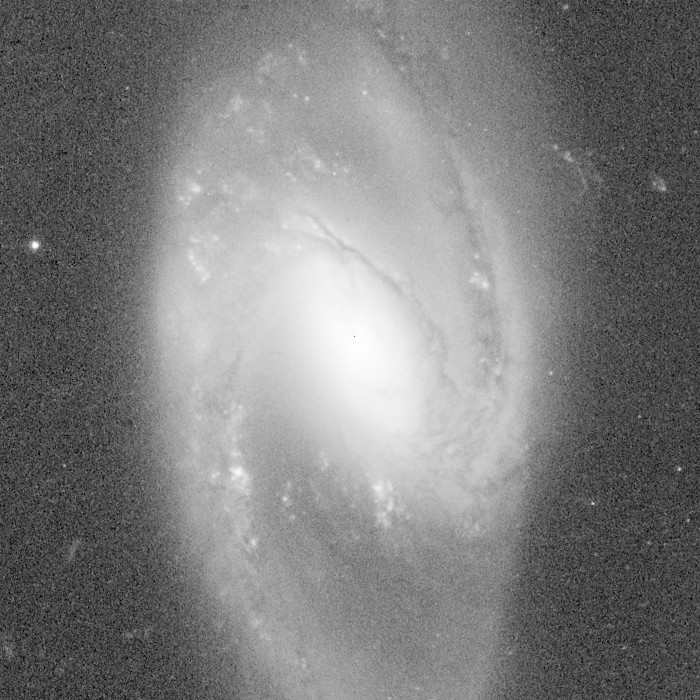
The core of the Arp 70 spiral at native resolution. Spiral arms, dust lanes and HII regions stay exactly where they are; only the grain between them goes. ES-WMV stopped this fit on its own at iteration 23 935.
Nothing here was sharpened or enhanced: the output is the raw linear result of the fit, displayed with the same stretch as the input.
 Input
DIPL
Input
DIPL
| Field | Stop iteration | Wall time |
|---|---|---|
| Arp 70 | 23 935 (early stop) | 4 h 52 |
| Arp 176 | 25 000 (cap) | 6 h 10 |
| Arp 180 | 18 124 (early stop) | 3 h 34 |
| Arp 255 | 14 605 (early stop) | 5 h 31 |
| Arp 293 | 18 000 (cap) | 6 h 32 |
HST ACS/WFC fields around 15 Mpx, one NVIDIA H200. The JSON sidecar
of every run (all parameters, the selected iteration, the timings) is published in the
repository under docs/runs/.
Run it on linear data after gradient removal (DBE), then blend, then stretch and finish as usual. The device is auto-detected: CUDA, Apple Silicon (MPS) or CPU, no flag to set.
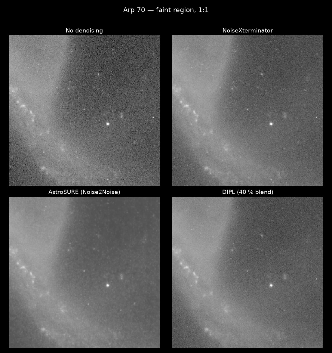
A faint region of Arp 70 at native resolution: no denoising, NoiseXterminator, AstroSURE (a Noise2Noise network trained on HST exposure pairs) and DIPL blended with the original. For a fair comparison every panel is brought to the same photometric frame and displayed with the same stretch, computed on the reference. NoiseXterminator is unbeatable on speed and excellent on ordinary fields. On faint diffuse structure, DIPL is the one I trust: there is nothing it could hallucinate from.